Requirements for self organization

What do you need to have a structure emerge spontaneously?

I am a Biologist

I am a ML researcher

I am a Physicist

Adaptive Abstract

This article is tailored to your preferences. Simply choose the researcher profile that resonates with you the most, and enjoy a personalized reading experience.

Feel free to join the discussion section to exchange ideas and offer feedback. Additionally, you have the opportunity to propose edits to the article in the discussion or issue section, or even by submitting a pull request. Your input is valued!

Abstract for Biologists

One of the most striking examples of self-organization is the formation of multicellular organisms, where most cells interact with their local environment through their cell membrane. The signals that each cell receives from its neighbors, and shifts in its own internal state, enable it to reach a specific cell type and self-regulate a variety of behaviors such as differentiation, proliferation, migration, and signaling. Despite the limited information available to each individual cell, incredibly complex organisms can be formed by cellular collectives. Crucially, the result is not just emergent complexity, but a kind of homeodynamic ability to take context-appropriate actions to reach the same large-scale form despite perturbations of internal components and external environment.

We have previously suggested that the ability of cell groups to traverse anatomical morphospace (during regulative development, regeneration, and cancer suppression) is a kind of unconventional problem-solving capacity that shares important features with other kinds of intelligence, such as familiar behavior and communication at the level of individual organisms.

In this work we show how the same process of self-organization that occurs in biological systems can be copied to improve narrative skills in linguistic space, where the words in a text self-organize to create a coherent whole. This is an important step towards characterizing the fundamental invariants that unify not merely the emergence of complexity, but goal-directed behavior, across diverse problem spaces and physical embodiments.

But what makes a system capable of self-organizing in the first place? In this paper we show that the ability of a system to self-organize relies on having the right topology for cell communication.

Furthermore, using tools from Statistical Physics, we propose that current state of the art architectures for text generation and biological brains lack the appropriate topology to be able to generate arbitrarily long, coherent output, and how organisms developed a habit of using the external environment to circumvent this problem. Thus, we show how exploring the symmetry of ideas between biology, physics, and computer science identifies important aspects of information-processing architectures relevant to diverse implementations.

Abstract for Physicists

One of the things that makes phase transitions beautiful is their universality. Despite the vast variety and complexity of systems of many particles, there are just a few of different phases of aggregation, and phase transitions are described by just a handful of critical exponents.

Furthermore, we observe that many systems tend to attain an ordered state at low temperatures. For instance, in Ising models, the ferromagnetic phase emerges with aligned spins, while materials exhibit a solid phase with a crystalline structure.

In this paper we are going to show that asking if it is possible to generate arbitrarily long, coherent text is equivalent to asking if the system is capable of having an ordered phase.

But what makes a system capable of self-organizing in the first place? In this paper we show that the ability of a system to self-organize relies on having the right topology for cell communication. Furthermore, we show that current state of the art architectures for text generation lack the appropriate topology to be able to generate arbitrarily long, coherent text.

Abstract for ML researchers

The complexity of generating a text with $N$ words using the Transformer architecture is $O(N^2)$ . This makes it computationally infeasible to generate coherent pieces of text as long as books. self-organizing systems, on the other hand, have two big strengths that transformers lack

• Efficiency: self-organizing systems often exhibit efficient resource allocation and optimization of processes. The emergent patterns and structures that arise from local interactions can lead to efficient distribution of tasks, information, or resources, resulting in overall system efficiency
• Scalability: self-organizing systems can often scale effectively. As the number of components increases the system can still organize itself without requiring additional centralized control. This property is valuable in various domains, such as computer networks, where scalability is crucial

Inspired from Biology and using tools from Statistical Physics we show that:

• Autoregressive models, no matter the architecture, the number of parameters, the window size, and the training procedure will never be able to generate text that is coherent at arbitrarily long distances.
• Transformers with attention matrices with a specifically crafted topology, can in principle be able to generate text that is coherent at arbitrarily long distances.
• An agent with a finite context size can be capable of enacting long term plans if it is able to interact with an external environment by deliberately storing and retrieving information.

Introduction for Biologists

Introduction for Physicists

Introduction for ML researchers

In many self-organizing systems, you see a hierarchical structures emerge

Advancements in machine learning technologies have brought about a revolution in various areas of biomedical research, by using AI as a tool to facilitate advancing existing paradigms in the field. However, can the exchange of ideas between biology and machine learning work both ways? Can insights from biology prove beneficial in the field of machine learning?

Specifically, can we find powerful invariants across domains - principles of system-level function which help to unify phenomena that have, until now, been treated as disparate sub-fields . The emerging discipline of “diverse intelligence” combines biology, computer science, and behavioral science to study the features common to active agents of very different provenance (evolved, engineered, and hybrid), material embodiment, and intelligence level .

A highly related concept is that of collective intelligence and swarm cognition , which is developing conceptual tools to help understand how evolution pivots and enlarges problem-solving capabilities of individual subunits into greater degrees of competency in larger problem spaces .

One of the most interesting aspects of biology is morphogenesis - the ability of cell groups to harness individual cell behaviors into reliable construction, repair, and maintenance of complex anatomical forms. We have recently argued that it is empirically fruitful to view this process not merely as emergence of complexity but as a kind of behavior (in anatomical morphospace) of a collective intelligence of cells which is able to solve a variety of problems .

This paper aims to showcase how the process of self-organization, observed in biological systems, can be harnessed to develop coherent narrative skills within linguistic space. By allowing words in a text to self-organize, a cohesive and meaningful whole can be created.

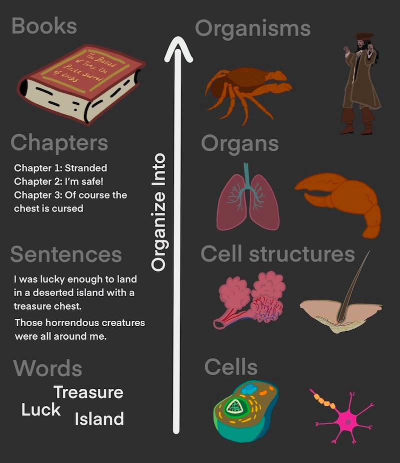
In textual context, words can organize themselves into sentences, which further organize into chapters, ultimately forming complete books, etc., as in biological organisms, cells organize into specific structures, which then combine to form organs, culminating in fully grown organisms and swarms

Certain machine learning algorithms, such as neural cellular automata, have shown remarkable ability to replicate aspects of the behavior of cells in biological organisms .

Here, we demonstrate that attempting to teach a machine learning algorithm to generate text by simply providing each word with information solely from its neighboring words is unsuccessful in achieving self-organization. In this paper we will prove that this is due to the fact that text is a 1-dimensional sequence of words, and self organization in 1D is impossible. Biological organisms are 3-dimensional so don't have this problem.

We also show that, in principle, it is possible to generate long-coherent text by making distant elements of text interact via long range connections.

Furthermore we demonstrate that biological brains are likely incapable of retaining memories forever, and thus many species, including humans, have developed skills that allow them to store information for long term by interacting with the external environment.
Thus, interacting with the external environment is something that is indispensable for long-term storage for all living beings.

These results support the consistent patterns we discussed earlier, highlighting the need for systems trying to store memories or maintain patterns to put that information into their environment. This need arises due to limitations in their self-organizing abilities. Using a generic model we prove that a large class of self-organizing systems face fundamental restrictions on how long they can maintain coherence, and can escape these limitations by writing information to a static environment. We follow up with examples like stigmergy and the human brain which fall under the “universality class” of self-organizational behavior described by this model.

Why focus on text to study self-organization?

• Long-range cohesion is a necessary feature of text, and it is something that current language processing algorithms don’t possess. This will mean that any improvement on the theoretical front, will directly translate into an application in the field of natural language processing.
• In text, spotting a misspelled word is easy. In biological (and virtual) organisms spotting an off place cell is hard.
  This raises the bar of difficulty so it will give a more rigorous test on the ability of self-organizing systems
• It’s easier to run experiments on code rather than biological organisms.
• Since text is a 1-dimensional sequence it can give insights into other types of 1D sequences, for example a sequence of actions performed by an agent.
  Having long term coherence for a sequence of actions performed by an agent means that the agent is able to stick to a plan and use information from the distant past to make decisions on what to do next.

Morphogenesis and Language Modelling

Side by side comparison between text generation and morphogenesis

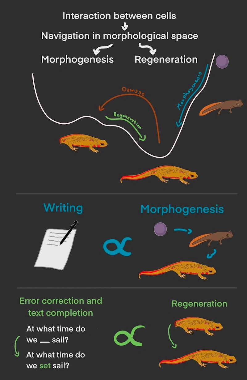
Many phenomena in self-organizing systems are interpreted in the literature as navigation in a morphological space. .

In various fields like biology, linguistics and computer science, a morphological space refers to a conceptual space where each point represents a specific configuration or form of an entity. The term "morphological" refers to the form, structure, or shape of something.

Navigating a morphological space involves exploring and moving through this conceptual space to observe or analyze the different configurations or forms that an entity can take. It is often used to understand the relationships between different variations or possibilities within a system. Better configurations are associated with a lower energy value, and the system evolves rolling down this energy landscape.

One common example is in biology, where the concept of morphological space can be used to describe the range of physical forms that a species can exhibit . By navigating this space, the organism changes shape over time. Both processes of morphogenesis and damage repair can be thought as navigating this morphological space towards the stable adult form of the organism. The damage becomes impossible to heal for the organism if it puts it in a point into the morphological space outside the basin of attraction of the stable configuration.

We propose that a number of biological phenomena, especially morphogenetic control, is a kind of navigation of a problem space (e.g., physiological, transcriptional, metabolic, and behavioral spaces) . This suggests a research program to understand what basic features of the organization of a swarm of subunits is necessary to enable efficient behavior of the system toward specific goals in various spaces, and potential applications driven by the use of basic biological principles to advance engineering and AI.

Drawing parallels between text generation and morphogenesis, text generation starts with a prompt (analogous to an embryo) and progresses, generating the rest of the text until completion. Similarly, correcting errors in text, such as misspelled or missing words, bears similarity to the process of cell level defects, and repairing damage in the whole organism can be associated with keeping a conversation on-topic. Both tasks are error correction procedures that involve navigating a morphological space to rectify errors and achieve the desired final state.

Specifically, we are interested in discovering the architectures needed to facilitate the kind of collective behavior that enables efficient competency of the collective, and deploying them in other domains. For our test case of moving across domains and exploring plasticity, we examined the parallels between maintaining a trajectory in morphospace (reliably creating a complex anatomy in novel circumstances) and maintaining a trajectory in linguistic space (keeping the thread of a coherent narrative).

The simplest example of self-organization: The Ising Model

Initially, when students delve into the study of the Ising model, they often find it utterly useless and struggle to comprehend why physicists are so fixated on this seemingly mundane model.

The problem is that it's hardly ever mentioned that the Ising model is key to understanding how self-organization works. This is because the Ising model is the simplest example of self-organization. Thus if you want to understand how more complex self-organizing systems work you have to start by understanding how the Ising model works.

But what exactly is the Ising model? Originally conceived as a simple explanation for magnetization effects in matter, the Ising model explores the interplay between interacting spins. These spins, when in proximity, have a preference to align with each other, leading to an interaction energy denoted by $H=-Js_1\cdot s_2$.

What happens when lots of spins interact? Well, it depends on how they interact: The Ising Model comes in many different flavors, we are going to look at the 3 simplest ones: the fully connected, the 1D and the 2D one.

Fully connected Ising model

In the fully connected Ising model we have L spins, all interacting with each other. The Hamiltonian of the system is $$H=-\frac JN\sum_{i\neq j}s_is_j$$ Now let’s see how the system behaves as a function of the temperature.

$T=$ 1.0

Simulation of the Fully connected Ising Model

As you can see, below a certain Critical Temperature $T_\textrm c$ you have an Ordered Phase, while above you have a Disordered Phase

1D Ising Model

In the 1D Ising Model, spins are arranged in a chain and interact with their neighboring spins. The system's Hamiltonian can be expressed as: $$ H=-J\sum_{i}s_is_{i+1} $$ Now, let's examine the behavior of this system in relation to temperature

$T=$

Simulation of the 1D Ising Model each spin interacts with the spin before and after. For space efficiency the spins have been put in a serpentine shape, as you can see even at low temperature the system stays unordered

As observed, regardless of how low the temperature is, the system never manages to achieve an ordered phase. This can be proven mathematically with the following theorem

Theorem

The 1D Ising chain doesn't have an ordered phase

proof

At thermal equilibrium, the Free Energy $F$ is minimized.This is because the Free Energy measures the amount of useful energy that can be extracted from a thermodynamic system. At thermal equilibrium, no useful energy can be extracted.

To demonstrate that the ordered state, where all spins align, is not the minimum of Free Energy, we have to examine what occurs when a domain wall forms.

The top image shows the ordered phase of the Ising model, while the bottom image depicts a state with a domain wall.

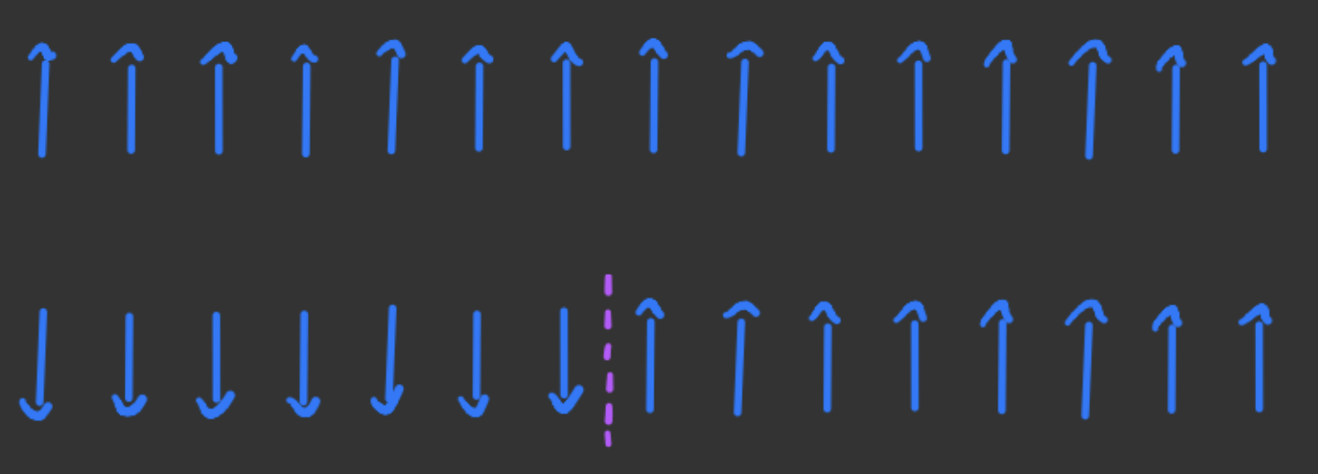
Upon the formation of a domain wall, the energy change increases by $2J$. This is because only a single link now comprises two opposite spins.

If the chain is $L$ spins long, there can be $L-1$ possible locations for the domain wall. Consequently, the size of the configuration space where a domain wall is present, denoted as $\Omega$, equals $\Omega = L-1$. Since entropy is the logarithm of the configuration space, we have $\Delta S = \log(L-1)$.

Therefore, the change in Free Energy upon the formation of a domain wall is given by: $$ \Delta F= \Delta E -T\Delta S= J - T\log(L-1) $$ In the thermodynamic limit, as $L$ approaches infinity, and since $J$ is a constant, we find that for any temperature $T$, $\Delta F < 0$.

Thus no matter how low the temperature (or the noise) is, it is impossible to reach an ordered state

2D Ising model

In the 2D Ising model the spins are arranged in a grid, and each one of them interacts with his neighbors. The system's Hamiltonian can be expressed as $$ H=-J\sum_{\langle i,j\rangle} s_is_j $$ Where $\langle i, j\rangle$ means that we sum over all the neighboring spins. And let's see how it behaves

$T=$ 1.0

Simulation of the 2D Ising model. If you hover over the image you the interaction window is displayed in orange. The critical temperature is at $T$=1

As you can see, when the temperature is sufficiently low, the system will slowly reach an ordered phase.

Theorem

The 2D Ising model does have an ordered phase

proof

The following proof is also known as Peierls Argument .

Suppose we start in a configuration where all the spins are all in the $+1$ configuration, we now create a domain with a perimeter $\mathcal P$ made of spins in the $-1$ configuration, and see what happens to the Free Energy.

The change in energy will be $$\Delta E= 2J\times \mathcal P$$ Where $J$ is the coupling strenght between spins

The change in Entropy is harder to estimate, fortunately we only need an upper bound.
We need to find the number of domain with a perimeter $\mathcal P$.

We can always fit a curve of perimeter $\mathcal P$ inside a box $\mathcal P\times \mathcal P$ centered in the origin, so the number of starting points is at most $\mathcal P^2$, then at each step along the perimeter the curve has at most 3 choices for where to step next, so for each starting point there are at most $3^{\mathcal P}$ curves The choices are usually less than 3 beacuse the curve is a close self-avoiding curve, so to satisfy this constraints usually has less choices. It can be proven that there are at least $2^{\mathcal P/2}$ possible configurations

We can thus conclude that the number of possible configuration $\Omega\le \mathcal P^23^\mathcal P$, and the change in entropy is $$ \Delta S\le \mathcal P\log3 +2\log\mathcal P $$ Putting it all toghether we have that $$\Delta F \ge 2J\mathcal P - T \mathcal P\log3 +O(\log \mathcal P)$$ And if $T$ is sufficently low we have that $\Delta F>0$, thus for low temperature the 2D Ising model at the equilibrium tends to an ordered phase.

However, there is a caveat here: The theorem doesn't tell us anything about how much time the system takes to reach equilibrium, in fact if the system is sufficiently large it can take more then the age of the universe. In this article we will not worry about the time it will need to reach equilibrium as this lays outside of the scope of this work.

If you want some great resources for learning about the Ising model and phase transitions in general I suggest you look at these books.

Ising model on a Tree

Many self-organizing systems seem to gravitate towards a hierarchical structure, in earlier sections of the paper we talked about how cells and words on the text organize into bigger and bigger structures. The same goes for how people organize into teams, companies, and so on.

So, let's take a briaf look at the Ising model on a Tree.
Interestingly, the Ising model on a tree can be thought as a 2D Ising model in hyperbolic geometry, this means that the same proof for the existence of an ordered phase is pretty much the same as the one in the 2D case, but with the extra flavor of hyperbolic geometry.

Ising model in a hyperbolic geometry. On the left the triangular hyperbolic lattice is equivalent to a tree with each 2 children nodes, on the right the pentagonal hyperbolic lattice is equivalent to the tree below FIND BETTER IMAGES

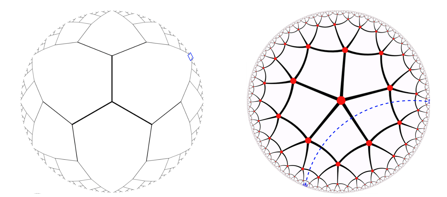
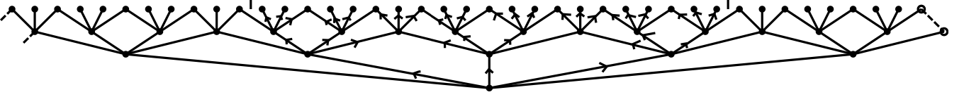
It does have the additional benefit that the average distance between a couple of spins in the same chain increases as $\log N$, so the information to go from one point to another needs to travel shorter distances.

Main takeaway from the Ising model

We have seen that the ability of a self-organizing system to reach an ordered state can indeed be understood through the lens of phase transitions. In fact developmental biology has studied this phenomenon in the context of planar polarity of cells in a 2D tissue , including the use of Ising models to understand collective decision-making in this patterning task.

When it comes to self-organizing systems, the concept of an ordered state typically refers to a highly organized and coherent configuration. For example, in the Ising model, an ordered state corresponds to spins aligning in a particular direction. In other self-organizing systems, it may involve patterns, structures, or coordinated behaviors emerging among the individual elements of the system.

Understanding the behavior of self-organizing systems in terms of phase transitions allows us to analyze their equilibrium properties, and gain insights into the underlying mechanisms driving the emergence of order. By studying the conditions and factors that influence phase transitions in self-organizing systems, we can better comprehend their ability to reach ordered states.

We will now give an overview of a more complicated self-organizing system through the lens of phase-transition: The Hopfield Network

Associative Memory

The brain is capable of storing and retrieving memories, but the way it does that is very different from how the memories are managed in a computer.

• Address based memories, which are the kind of memories stored in a computer, work that given a memory address, it gives you back the information stored in that specific address.
• Associative memories are how memories are stored and extracted in human brains. In an associative memory system, when given an input, the system returns the most associated memory it has stored; furthermore a memory becomes easier to extract the more “hints” or related memories are given.

An example of associative memories are search engines. What a search engine does is to return the most associated results to the query given by the user.

In general, a associative memory can be modeled as a energy landscape with with a discrete number of minima, each of which corresponding to a stored memory

Example of associative memory, in this case each member of the Simpsons family has his own enegry minimum. When given a guess of the system will converge to the closest Simpsons member. Images adapted from .

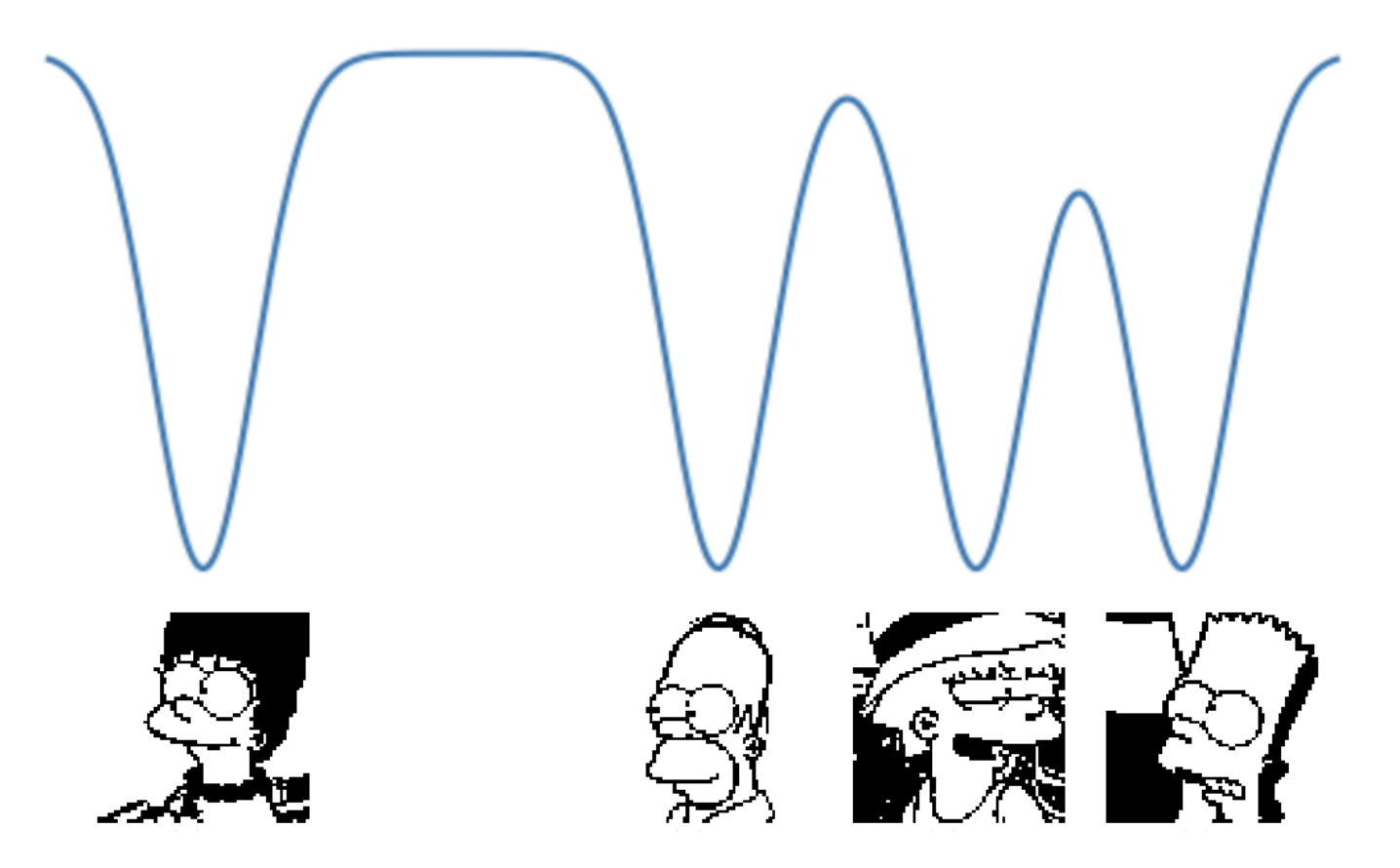
Associative memories, just like the memory inside a computer, have finite capacity. How do we quantify this?
Intuitively what ends up happening when you try to store too many separate memories, is that the configuration space becomes too crammed and some of the saved patterns fuse together.

Example of a saturated associative memory, when lots of patterns are stored, minima that are close together fuse and are no longer distinguishable. Images adapted from .

Hopfield Networks

Hopfield Networks are one of the most famous examples of associative memories, and, it turns out that, when generalized, they are equivalent to the Transformer architecture . It is the perfect working bench to understand what are the capabilities of associative memories.

The standard Hopfield Network with $N$ patterns stored equation is the following $$ H=-\sum_{ij}W_{ij}s_is_j\quad\textrm{ with }\quad W_{ij}=\sum_p^NX^p_{i}X^p_{j} $$ Notice how this is similar to the equation of the Hamiltonian of the fully connected Ising model ...Actually if there is just one stored pattern they are equivalent up to a Gauge transformation $s_i\to X_is_i$. What effectively does is that it creates a number of local minima equal to the number of patterns stored, here is a simulation.

$T=$ 1.0

Here is a simulation of the Hopfield model, the two patterns stored are a image of Homer and Marge Simpsons
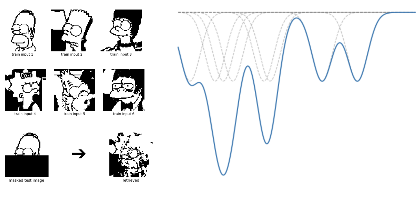
You can go from a saved pattern to the other by increasing the temperature and relowering (it works 50% of the times). If you dont want to wait for the system to thermalize you can just reload the page.

As you can see at low temperature the system converges to the closest state, but at high temperature the system is noisy.

Hopfield networks with local interaction

Many of the self-organizing systems in real life are capable of reaching a highly ordered state even with just local interactions, so what happens if the Hamiltonian of the Hopfield network makes spins interact only if they are close by? $$ H=-\sum_{\langle i,j\rangle}W_{ij}s_is_j\quad\textrm{ with }\quad W_{ij}=\sum_p^NX^p_{i}X^p_{j} $$ In this case $\langle i,j\rangle$ means that $i$ and $j$ are in the same window of interaction. Here is a simulation to play with.

$T=$ 1.0 $W=$ 5

Example of a Hopfiled network with just local interaction. By hovering the mouse over the figure you can see all the interaction windows. You can set the size of the interaction windows $W$ by moving the relative slider.

As you can see the system struggles more to converge to one of the saved patterns, and the smaller the window size is, the harder it becomes.
What is possible to conclude even with this small demo is that the memory capacity of a local Hopfield model is lower, we will later analyze by how much.

What makes a self-organizing system capable of organizing?

So far we have seen that

• The 1D Ising model is not capable of self-organizing in to an ordered phase
• The 2D Ising model is capable of self-organizing in to an ordered phase, but it takes time
• The Fully connected Ising model is capable of self-organizing in to an ordered phase and it does that quickly
• The Standard Hopfield Network, which is a generalization of the Fully connected Ising model is capable of self-organizing quicky, but it doesn't have a large memory capacity
• Windowed Hopfield wich are a generalization of the 2D Ising model are in principle capable of self organizing, but their memory capacity is lower than the one of standard Hopfield Networks, and it takes time to self-organize

But is there a unified way of determining if any system is capable of self organizing?

It turns out that a system can be capable of self-organizing if it is topologically equivalent to an Ising model which has a condensed phase at low temperatures.

It turns out that there is, but before proving in the general case, we will first prove why autoregressive models for text are incapable of generating text that remains coherent at arbitrary lenghts as it gives us the intuition to prove it in the more general case.

Topological requirements for self-organization

First, we generalize the value that the spins can take: instead of $-1$ and $1$, they can now take any integer value from $0$ to $V$For now we are going to ignore the possibility of having continous valued elements

The 1D case Definition: Potts Chain

A Potts chain is $\mathcal C$ chain of spins $s_i$ with $i \in \mathbb{Z}$ and each $s_i$ can assume any integer value from $1$ to the vocabulary size $V$

Ok, now we are going to define how this new spins interact with one onother. We want them to interact with only their neighbours, thus only interactions inside a finite Window are non zero.

Definition: Hamiltonian Window

A Hamiltonian window $H_i$ is an Hamiltonian that acts only on the spins inside his finite window of interaction $\mathcal W_i$. Without loss of generality, we are going to assume that the lowest energy state has a value of zero.

Definition: Local Hamiltonian

A Local Hamiltonian $H=\sum_i H_i$ is an Hamiltonian that can be written as the sum of several windowed Hamiltonians $H_i$ all with the same window width $\mathcal W$. For sake of simplicity we are going to assume that there exists an upper bound to the highest energy of every windowed Hamiltonian $E^\textrm{max}_i < E^\textrm{max}$

The time evolution of this chain is governed by a local Hamiltonian which is the sum of several Hamiltonian windows, you can see all the Hamiltonian windows by hovering on top of the chain elements. In this case the elements of the sequence interact in groups of five.

As you can see this is a very general structure that can be used to model cells, agents, particles, and words arranged in a line or evolving though time.
Ok, now what is a memory in this kind of situation? A pattern stored is a particular configutation of spins with zero energy, or more precisely:

Definition: Memory or Pattern stored

A stored pattern $\mathcal P$ is a particular sequence of spins $(\dots, s_{-1}, s_0, s_1,\dots )$ such that the energy of the Hamiltonian $H$ associated to this pattern is equal to zero. If more than one stored pattern is present, they can be numbered as $\mathcal P^{(n)}$ = $(\dots,s^{(n)}_1,s^{(n)}_0,s^{(n)}_1,\dots)$.

Notice how we don't really care what the spins represent: They can be the words in a text, or the state of the cells of an organism, or the actions performed by an agent, or the value of a title in the stock market.
We also don't really care how the values of the Hamiltonian are evaluated: The architecture of the model doesn't matter.

We are now going to prove that local Hamiltonians in 1D, no matter how low the temperature, cannot have a condensed phase.

Theorem

Let $H$ be a local Hamiltonian with $N$ > 1 stored patterns. At non-zero temperature the system will be unable to converge to single stored pattern.

proof

Suppose that our Potts chain starts out equal to our first stored pattern $\mathcal C=\mathcal P^1$. Now we want to know if the formation of a single domain barrier is thermodynamically favorable. $$ \Delta F=\Delta E -T\Delta S< 0 $$ For that to be true, the Free energy of the system must decrease upon the formation of a domain barrier. Upon the formation of a domain barrier, The windowed Hamiltonians that intersect it will have a non zero, positive energy. Therefore $\Delta E >0$, however, we know that the energy of each window Hamiltonian is smaller than $E^\textrm{max}$ and no more that $\mathcal W-1$ windows can be affected by a domain wall, therefore $$ 0\le\Delta E\le (\mathcal W-1)E^\textrm{max} $$ At the same time we know that in a sequence long $L$ there can be $L-1$ possible places where a domain wall can appear, and for each of this possible places it can lead to any of the $N-1$ other patterns saved, therefore there are $(L-1)(N-1)$ possible configurations where the system has a single domain wall. This means that the change of the entropy of the system is $$ \Delta S=\log [(N-1)(L-1)] $$ Putting all the equations together we have that $$ \Delta F\le (\mathcal W-1)E^\textrm{max} - T\log [(N-1)(L-1)] $$ In the thermodynamic limit ($L\to \infty$) we have that the right hand side of the equation becomes eventually negative, therefore the domain barriers are inevitable.

We have now seen that 1-dimensional self-organizing systems can't really existsWe are assuming that there are at least two different ground states, .

Autoregressive models Definition: Autoregressive Model

Given some input tokens $\{s_{i_\textrm{first}},\dots, s_{i_\textrm{last}}\}$ an auto-regressive model $M$ return a $V$-dimensional $(p_1,\dots,p_V)$ vector with an estimate of the probability for the next element in the sequence $i_\textrm{pred}=i_\textrm{last}+1$ $$ p_c=M(s_{i_\textrm{pred}}=c|s_{i_\textrm{first}},\dots,s_{i_\textrm{last}}) $$ where $p_c$ is the porbability that the next spin $s_{i_\textrm{pred}}$ is equal to the $c$-th token of the vocabulary

$T=$ 1.0

Simulation of an autoregressive Ising model. In this example to predict the next element in the sequence $s_{i+1}$ the model only looks at the last known element of the sequence $s_i$, and the vector with a estimate of the probability for $s_{i+1}$ is just a 1-dimensional vector equal to $p=\left(1+e^{J/T}\right)^{-1}$. We can write the Hamiltonian windows of the system wich are equal to $H_t=-Js_ts_{t+1}$

We will now make the parallelism explicit with Natural Language Processing. Most state of the art language models of today are Autoregressive, meaning to predict the next word (or token) they look at all the previous elements on the text.
However, as the context increases, it becomes computationally infeasible to predict the next token, and only the last few words are fed as input to the model.

Intuitively, this leads the model to completely forget what is left outside of its input window

Keep in mind that how well you can predict the next element in a senquence can be considered a measure of intelligence. After all, what any intelligent agent does is just finding the best next action.

But how do we prove mathematically that autoregressive models with finite context are bound to lose the thread?
We show that Autoregressive models, no matter the architecture, are equivalent to a thermodynamic system with a specifically crafted local Hamiltonian

The significance of demonstrating the incapability of autoregressive models doesn't lie solely in the theorem itself. Intuitively, we already understand that autoregressive models, due to their inherent loss of information over time, are unable to generate lengthy texts. What holds importance is that through mathematical proof, we gain the knowledge necessary to establish the coherence of text generation through alternative methods.

Theorem

It is possible to associate local Hamiltonian to any auto-regressive model

proof

Let $M$ be out autoregressive model, and $s_{i_\textrm{first}},\dots,s_{i_\textrm{last}}$ our input sequence. then the probability that the next token in the sequence is equal to $c$ is. $$ p_c=M(s_{i_\textrm{pred}}=c|s_{i_\textrm{first}},\dots,s_{i_\textrm{last}}) $$ Through Boltzmann's equation it's possible to turn a probability distribution to some energy levels $$ p_c=\frac 1Ze^{-\frac{E_c}{T}}\quad\textrm{with}\quad c=1\dots V $$ Without loss of generality, we can assume $T=1$ and set the energy associated with every prediction turns out to be $$ E_c=-\log p_c +\textrm{const} \quad\textrm{with}\quad c=1\dots V $$ Where we can set the constant in such a way that the lowest energy state has a energy equal to zero.
We can now define a windowed Hamiltonian $$ H_{i_\textrm{pred}}(s_{i_\textrm{first}},\dots,s_{i_\textrm{last}},s_{i_\textrm{pred}})=-\log\left[ M(s_{i_\textrm{pred}}|s_{i_\textrm{first}},\dots,s_{i_\textrm{last}})\right]+\textrm{const} $$ And the full local Hamiltonian can now be seen as the sum of all the $H=\sum H_{i_\textrm{pred}}$ of the sequence.
The generation process of an autoregressive model can now be seen as sampling from the Boltzmann distribution given from $$ p_\textrm{sequence}=\frac 1Z e^{-\frac 1TH(\textrm{sequence})} $$

So, we now know that autoregressive data generation is equivalent to sampling form the Boltzmann distribution of a local Hamiltonian (usually at $T\approx 1$), and since 1-dimensional local Hamiltonians are inherently unstable it means that autoregressive models with a finite context window are too.

More complex Topologies

As you have seen from the examples, determining whether or not an ordered phase can exists boils down to a counting problem.

1. Start with the system being equal to one of the patterns stored
2. Create a domain wall
3. Count the number of such domain walls
4. Estimate the energy gained by the system
5. See if there exists a finite temperature for which the free energy decreases as the size of the domain walls goes to infinity

This can be applied to systems with very different topologies, we are now going to explore that

The most general way to consider the interaction between the elements of our system is if the interactions are represented by a graph Hamiltonian

For simplicity we are going to consider that the links of the graph are fixed in time. This is a simplification and loads of self-organizing systems have a interaction graph that changes with time, for example most of the people you interact daily are different from the people you interacted in your childhood.
Sometimes even the topology of the entire graph changes, for example before the invention of means of rapid communication each person interacted only with the people nearby thus the topology was 2-dimensional. Today, with the internet we can interact with people far away.
However, we can say that even though the interaction graph changes with time, it usually changes slowly relative to the dynamics of the time evolution of its elements.

Definition: Graph Hamiltonian

Let G be the adjacency matrix of a graph, then a Graph Hamiltoninan H is a Hamiltonian that can be written as $$H=H*G$$ where the ($*$) operator is the element wise multiplication.

Now to see if a ordered phase can ever exist, we must generalize Peierls argument. To see if an ordered phase exists we only care how the enegry and the entropy increase when we create a domain wall

Definition: Entropy Scaling

Let $H$ be a Graph Hamiltonian, and $P$ be the perimeter length, or surface area of a domain wall, as the perimeter length increases, the number of possible configurations of domain barrier increases, thus increasing the entropy of the system $\Delta S$. We say that the Entropy gained scales as $f_S$ if \[ \Delta S=O(f_S(P)) \]

Definition: Energy Scaling

Let H be a Graph Hamiltonian, and $P$ be the perimeter length, or surface area of a domain wall, as the perimeter length increases, the the Higher and Lower bound of the energy gained $\Delta E$ scale as respectively $O(f_E^\textrm{high}(P))$ and $O(f_E^\textrm{low}(P))$. If $f_E^\textrm{high}=f_E^\textrm{low}\equiv f_E$ we say that the energy gained scales as $f_E$ \[ \Delta E=O(f_E(P)) \]

Once we know how the entropy and the energy scale, we know if there is a ordered phase

Theorem

If $O(f_S)=O(f_E)$ there exists a ordered phase

proof

Let's define $O(f)=O(f_S)=O(f_E)$, the change in Free energy is now $$ \Delta F= \Delta E -T\Delta S=\lim_{P\to \infty}O(f(P))-TO(f(P)) $$ If we now do $\lim_{T\to0}$ the term on the right disappears, therefore the creation of a domain wall increases the free energy and so a coherent phase is favored

This means that we don't really care about the exact formula for $E(P)$ and $S(P)$, but only on how they scale as $P\to \infty$, so we can rule out some details that can lead to complications, for example the number of stored patterns

Theorem

Let $H$ be a Graph Hamiltonian with $N>1$ stored patterns. At thermal equilibrium, the ability to converge to a ordered phase doesn't depend on $N$

proof

The change in entropy due to the creation of a domain barrier can always be written as $$ \Delta S= \log\left[ (N-1)N_\textrm{barriers}\right]=\log N_\textrm{barriers} + \log (N-1) $$ Where $N_\textrm{barriers}$ is the number of barriers of a certain shape. In the thermodynamic limit, the term proportional to the number of barriers increases, while the one proportional to the number of patterns stored stays constant, therefore can be ignored as it doesn't change the entropy scaling

The importance of this last theorem is that, since the number and the shape of stored pattern doesn't affect the thermodynamics of the problem we might as well stick with a system with just 2 ground state equal to all spin ups and all spin downs. Like in the Ising Model!
We are also go one step furter we can also show that we don't really care on how strong, complicated the interaction are, and neither on how big the interaction windows are.

Theorem

Let $H=\sum_i H_i$, if there exists two energies $E_\textrm{max},E_\textrm{min}$ which are the biggest and smallest non-zero energy level of all the windowed Hamiltonians $H_i$. At thermal equilibrium, the ability to converge to a ordered phase does not depend from the energy levels and the window sizes

proof

Let $\mathcal W$ be the biggest window size, and 1 the smallest window size of any $H_i$, and let $P$ be the perimeter length of our domain wall. The energy gain by creating such a domain wall is bounded by $$ P E^\textrm{min}\le\Delta E\le \mathcal W PE^\textrm {max} $$ In both cases we have that $$ E=O(P) $$

This means that, even if we have a really complicated local Hamiltonian, with large window sizes, large vocabulary size and many patterns stored, we can just look at a simple next-neighbour Ising model to see if we have a coherent phase

Main Takeaway

In this section we saw how the only thing that matters to determine if a system can be capable of self organizing at thermal equilibrium is the topology of the system.

This also means that to see if a system has the required topology to have an ordered phase you need to make sure that a topologically equivalent Ising model has an ordered phase.

The role of Disorder

In all the theorems we saw, we assumed that the Free energy is minimized. This is true at thermal equilibrium, however for some systems the time it can take to reach thermal equilibrium can be larger than the age of the universe.

Example of a rugged energy landscape. The system to reach the global minimum will take a really long time. Courtesy of

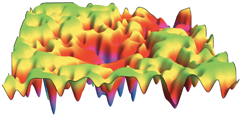
This usually happens when the energy landscape is rugged. Essentially the system stays trapped in a local minima before it ever gets the chance to get to one of the global minima. In the rare occurrence that the system manages to escape the local minimum it will most likely go to another local minimum.

When a system is like this we say that it is a spin-glass system.

A spin glass system is a type of physical system that exhibits what's called "quenched disorder." This disorder arises due to random couplings, denoted as $\theta$ among the different degrees of freedom within the system, which are represented by the variable $s$. The disorder is explicitly incorporated into the Hamiltonian of the system, and is completely specified by its probability distribution, $p(\theta) d\theta$. $$ H=H(\theta,s) $$ One of the most well-known examples of such a system is the Edwards-Anderson model , which is a finite dimensional model where the spins, represented by $s$, are the degrees of freedom and the couplings, represented by $\theta_{ij}$, are Gaussian random variables. $$ H=-\sum_{\langle ij\rangle}J_{ij}s_is_j $$ In this model, the sum is performed over nearest-neighbor spins. The disorder is said to be "quenched" because the $\theta$ values remain constant over the timescale during which the $s$ values fluctuate. Spin-glass systems are frequently found in machine learning algorithms. For example lets say our system searches trough a family of Hamiltonians dependent from a set of parameters $\theta$, then the Free energy will depend on theta as such $$ F(\theta)=-T\log\left[\int e^{-H(\{s_i\}|\theta)/T}Ds_i\right] $$ However different parameters will yield give different free energies, and since they are learned they follow a distribution $p(\theta|\mathcal D)$ dependent on the dataset $\mathcal D$. A more meaningful variable will be the expected free energy $\langle F\rangle$ $$ \langle F\rangle=\int F(\theta)p(\theta|\mathcal D)d\theta $$ Since the loss function is the negative log likelyhood of the parameters $l(\theta|\mathcal D)=-\log p(\theta|\mathcal D)$ we can combine this with the last two equations to get $$ F=-T\int e^{-l(\theta|\mathcal D)}\log\left[\int e^{-H(\{s_i\}|\theta)/T}Ds_i\right] D\theta $$ This systems, more often than not, exhibit glassy behaviors, and as such, must be treated with extra care.

But how can we make sure that our self organizing system behaves more like an Ising model, and not like a completely disordered spin glass? For Hopfield models people have figured it out.

Memory of an Hopfield model

Phase diagram of the Hopfield Network. On the $y$ axis we have the temperature, and on the $x$ axis we have $\alpha=N/D$ where $N$ is the number of indipendent patterns stored and $D$ is the number of pixels.
Courtesy of

An Hopfield model with one pattern stored is mathematically equivalent to the Ising model.
As you add more and more patterns it starts being more and more difficult for the system to converge to any given pattern, until it can't take it no more and it becomes glassy.

But how many patterns can our system have before it becomes glassy?

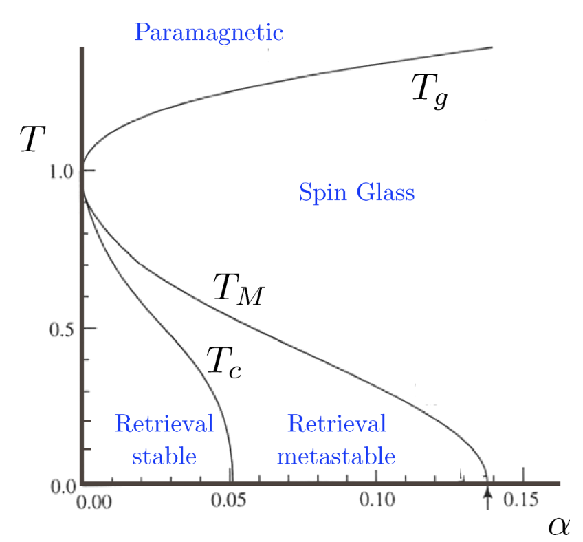
The statistics of this system have been extensively studied in the literature and can be schematized in the phase diagram.

It has been shown that the total number of patterns N that it is possible to store in this kind of memory is $N\approx 0.14\times P$. This estimate assumes that the patterns are statistically independent. For real life data this is usually not true as the patterns are hardly ever statistically independent, so it should be taken as an upper bound.
Studying the phase diagram rigorously can be challenging, but there are some less rigorous ways that are good enough and are much easier to generalize.

In the authors proved this theorem

Theorem

Let $H$ be a dense Hopfield network described by the following Hamiltoninan $$ H=-\sum_p^N F\left(\sum_i X^p_is_i \right) $$ Where $X^p$ is the $p$-th saved pattern.
If $F(x)=x^n$ with $n$ even the storage capacity increases with $L$ as $\alpha_n L^{n-1}$, where $\alpha_n$ is a constant dependent on $n$ and the Hamiltonian can be re-written as

outline of the proof

This is not the full proof, as that can be found in the original paper , what we really care here is the main idea.

We need to estimate the probability that at least one of the patterns is unstable

1. Take with a system with $N$ random indipendently sampled patterns saved $\{X^p\}_{p\in \{1,\dots,N\}}$
2. Choose as a starting configuration equal to one of the patterns saved $s_i=X^q$
3. To see if the pattern saved is a local minimum, perturb the system by flipping one bit. If the energy decreases ($\Delta E < 0$), then its not a local minimum $$ \Delta E = \sum_{p}^NF\left( X^p_iX^q_i+\sum_j^D X^p_iX^q_i \right)-\sum_{p}^NF\left( -X^p_iX^q_i+\sum_j^D X^p_iX^q_i \right) $$
4. Evaluate the mean $\langle \Delta E \rangle$ and the standard deviation $\Sigma^2=\langle \Delta E^2\rangle - \langle \Delta E\rangle^2$ of the change in energy over all the possible starting configurations $\{X^p\}_{p\in \{1,\dots,N\}}$
5. Estimate the probability that the energy change is negative by assuming that the probablity distribution of $\Delta E$ is a gaussian of mean $\langle \Delta E \rangle$ and the standard deviation $\Sigma^2$ $$ P_\textrm{error}=\int_{\Delta E}^\infty\frac 1{\sqrt{2\pi \Sigma^2}}e^{-\frac{x^2}{2\Sigma^2}}dx $$

Similarly, in the authors proved that if $F(x)\approx e^x$ the the storage capacity goes like $e^{\alpha L}$.
Their proof is more rigorous, but the main idea is the same.

Local Hopfield Networks

While these techniques are effective in increasing the memory capacity of the Hopfield network, each spin effectively interacts with every other spin. What we want is a system that is capable of self-organizing with just local interactions.

Let's define a generalized Hopfield Network where all the interactions are local.

Definition: Local Hopfield Network

The Hamiltonian of a windowed Hopfield networks is a sum over many Hopfield networks, each of which interacts inside its own window $$ H=-\sum_j^L\sum_p^NF\left( \sum_{\langle i,j\rangle}X^p_i\sigma_i \right) $$ If $F(x)=x^n$ or some other polinomial of $n$-th grade, the Hamiltonian above can be written as $$ H=-\sum_{\langle i_1,\dots,i_n\rangle}W_{i_1,\dots,i_n}\sigma_{i_1}\dots\sigma_{i_n} $$ Where $\sum_{\langle i_1,\dots,i_n\rangle}$ means that we are summing over all possible combinations of $n$ spins that are inside the same window of interaction.
A nice way to imagine local Hopfield network is as a patchwork of several overlapping Hopfield networks

Previously we have already seen a simulation of a local Hopfield Network with pairwise interactions.

Now that all interaction are inside a certain window, how does it change the number of stored patterns? Weirdly the memory capacity of local Hopfield network does not depend on the total number of elements, instead it is only dependent on the window size of the interactions.

Theorem

The memory capacity of a local Hopfield network with a window size equal to $\mathcal W$ is equal to the memory capacity of a standard Hopfield network with $\mathcal W$ elements.

Proof

Similarly to the theorems in we are going to start the system with every spin equal to one pattern saved at random $X^q$, and then perturb perturb the system in the position $k$.
The difference in energy is equal to $$ \Delta E=\sum_{\langle j,k\rangle}\sum_p^N F\left(X^p_kX^q_k+ \sum_{\langle i,j\rangle\neq k}X^p_iX^q_i \right)- F\left(-X^p_kX^q_k+ \sum_{\langle i,j\rangle\neq k}X^p_iX^q_i \right) $$ The reason why the first summation is only for the spins $j$ neighboring $k$ is because only Hamiltonian windows that have the spin $k$ inside them are direcly influenced by the spin flip.

To make the calculations easier, we are going to define the local change in energy, which by how much the Hamiltonian window centered in $j$ changes his energy when the spin $k$ is flipped. $$ \Delta E_\textrm{loc}(j)\equiv \sum_p^N F\left(X^p_kX^q_k+ \sum_{\langle i,j\rangle\neq k}X^p_iX^q_i \right)- F\left(-X^p_kX^q_k+ \sum_{\langle i,j\rangle\neq k}X^p_iX^q_i \right) $$ We can now write the total difference in energy as $$ \Delta E=\sum_{\langle j,k\rangle}\Delta E_\textrm{loc}(j) $$ When averaging over all the possible patterns $\{X^p\}_{p\in\{1,\dots,N\}}$ the $j$ dependence goes away.
This means that the average energy change of the local Hamiltonian is $$ \left \langle \Delta E \right\rangle = \sum_{\langle j,k\rangle} \left \langle \Delta E \right\rangle_\textrm{loc}=W \left \langle \Delta E \right\rangle_\textrm{loc} $$ Now we calculate the variances, first the change in energy can be written as $$ \Delta E^2=\sum_{\left \langle j_1,k \right\rangle} \sum_{\left \langle j_2,k \right\rangle}\Delta E_\textrm{loc}(j_1)\Delta E_\textrm{loc}(j_2) $$ Now we calculate the average of the term inside the sum.
When we flip a bit in one window, the change in energy in the other window will be close to it. $$ \Delta E_\textrm{loc}(j_2)=\Delta E_\textrm{loc}(j_1) + \delta $$ Where $\delta$ is a random variable independent from $\Delta E_\textrm{loc}(j_1)$How really accurate is this? I'm sure that if there is a dependence it is going to be small, should we consider it? and how?.
Since on average the energy change of the window centered in $j_1$ is the same as the one centered in $j_2$ $$ \left \langle \Delta E_\textrm{loc}(j_1)\right \rangle=\left \langle \Delta E_\textrm{loc}(j_2)\right \rangle $$ we have that $\left \langle \delta \right \rangle=0$ This means that $$ \begin{split} \left \langle \Delta E_\textrm{loc}(j_1)\Delta E_\textrm{loc}(j_2)\right \rangle=&\left \langle \Delta E_\textrm{loc}^2(j_1)\right \rangle + \left \langle \Delta E_\textrm{loc}(j_1)\delta\right \rangle =\\ =&\left \langle \Delta E_\textrm{loc}^2\right \rangle+\left \langle \Delta E_\textrm{loc}(j_1)\right \rangle\left \langle \delta\right \rangle=\\ =&\left \langle \Delta E^2_\textrm{loc}\right \rangle \end{split} $$ Where from the first to the second row we have used the fact that $\delta$ is independent from $\Delta E_\textrm{loc}(j_1)$, and form the second to the third row we have used the fact that $\left \langle \delta \right \rangle =0$.
Therefore equation $\Delta E^2$ becomes $$ \left \langle \Delta E^2\right \rangle=W^2\left \langle \Delta E^2_\textrm{loc}\right \rangle $$ and the variance is $$ \Sigma^2=W^2\left(\left \langle \Delta E^2_\textrm{loc}\right \rangle - \left \langle \Delta E_\textrm{loc}\right \rangle ^2\right)=W^2\Sigma_\textrm{loc} $$ Suppose that the probability distribution is a Gaussian with mean $\left \langle \Delta E\right \rangle$ and variance $\Sigma^2$. Then the probability of making an error is the probability that after the spin flips, the energy of the system decreases. $$ \begin{split} P=&\int_{\Delta E}^\infty\frac 1{\sqrt{2\pi\Sigma^2}}e^{-\frac{x^2}{2\Sigma^2}}dx=\\ =& \int_{W\Delta E_\textrm{loc}}^\infty\frac 1{\sqrt{2\pi W^2\Sigma_\textrm{loc}^2}}e^{-\frac{x^2}{2W^2\Sigma_\textrm{loc}^2}}dx=\\ =&\int_{\Delta E_\textrm{loc}}^\infty\frac 1{\sqrt{2\pi \Sigma_\textrm{loc}^2}}e^{-\frac{z^2}{2\Sigma_\textrm{loc}^2}}dz=\\ =&P_\textrm{loc} \end{split} $$ Where in the last passage we defined $z=x/W$.

This means that a Hopfield network with an energy function that is the sum of several overlapping sub-Hopfield networks with window size of $W$ has a storage capacity of any given sub-network

This is the main result of the paper: It shows us how complex and intelligent can be a self-organizing system made of just local interactions (assuming that the topology of the system allows for an ordered phase to exist)

It is crucial to bear in mind that these represent some of the essential prerequisites.
Similar to how possessing Turing Completeness does not guarantee intelligence, having an ordered phase in a system does not automatically imply that the output will be actually coherent and meaningful.

We now possess all the necessary elements to ascertain whether a system can ever exhibit the capacity to generate data coherently.

1. Select a topology of communication of the cells that is equivalent to an Ising model that has an ordered phase
2. Make sure that the system in not bottlenecked by the memory capacity (either by having a large enough window size and a large enough number of trainable parameters)

Now let's see some examples form the literature

Some practical examples Tree language model

We want to see if a transformer that has an attention matrix with the topology of a tree can ever generate text.

• Since the Ising model on the tree does have an ordered phase ,the possibility of generating an infinitely long, coherent text is not constrained by the topology
• The bottleneck provided by the memory capacity can be widened by increasing the window size and the number of parameters

Experiments

Recently a paper has come out that uses a tree-like attention structure where the authors were able to generate text that has a linear complexity and an effective context size of 1 billion tokens.

Building blocks of dilated attention used in LONGNET. It consists of a series of attention patterns for modeling both short-range and long-range dependency. The number of attention patterns can be extended according to the sequence length. Courtesy of

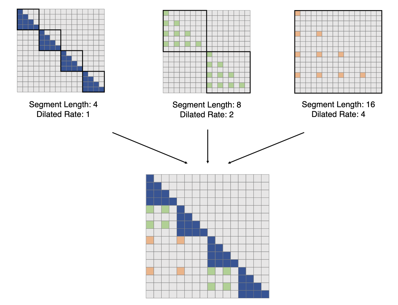
However, it is unclear if this specific experiment resulted in a model that is actually capable of retrieving any information inside that effective context of 1 billion tokens.

Brain + Environment

Let's start with a system inspired by how the brain is thought to work.

One can naively say that the way the state of the brain at the time $t$ depends from the state $t-1$We are assuming the time to be discretized, but this can be easily generalized $$ B_{t+1}=f_B(B_t) $$ This effectively makes the brain an autoregressive model, thus it is incapable of retaining information for an indefinite amount of time. On one hand, we human beings do forget lots of things, but on the other hand we seem to be able to also have long-term memory and the ability to stick to a plan for even decades.

However we (and some other organisms) also augment our finite memory by deliberately interacting with the environment, this way we are able to remember stuff for much longer.

For example when you go shopping, you write down what you have to buy on a piece of paper, this is because information stays there longer and more reliably than if you try to remember it.
This example also raises an interesting observation: When you read your shopping list, you effectively "interact" with your past self though interacting with a piece of paper memories, whether internal or on paper, are messages or prompts from your past self. In some sense we can say that effectively $B(t_\textrm{s})=B(t_\textrm{h})$ where $t_\textrm{s}$ is when you are at the supermaket, and $t_\textrm{h}$ is when you are at home writing the shopping list.

Diagramatic representation of brain-environment interaction

This sort of thing happens all the time, our brain constantly interacts with the surrounding environment so much that it is impossible to study the brain independently from the environment And reconstructs its state from engrams available to it as such a thing doesn't exist. This concept echoes the extended mind thesis, a perspective that suggests our cognitive processes are intricately linked with our environment. According to this view, the study of the brain cannot be divorced from its ongoing interaction with the surrounding world, as it challenges the idea of a self-contained, isolated brain, highlighting the significant influence of external factors and tools on human cognition.

We humans are not the only ones engaged in this intricate dance of information exchange with their environment. Nature has its own fascinating mechanisms for information storage and communication, one of which is known as "stigmergy" . For example ants leave pheromone traces or signals in their environment as they go about their tasks. When a group of foraging ants discovers a food source, they lay down a chemical pheromone trail on their way back to the colony. As a result, the rest of the colony is more likely to find and follow the trail to the food source.

Now let's look at the brain+environment system from a more formal point of view.

Let $B_t$ be the state of the brain at the time $t$ and $E_t$ the state of the environment, we can say that the way they evolve is ruled by a set of equations like this. $$ \begin{cases} B_{t+1}=f_B(B_t,E_t)\\ E_{t+1}=f_E(B_t,E_t) \end{cases} $$ Note that this is simply an autoregressive model made of two coupled autoregressive models, however we can assume that the environment is capable of holding on to information for longer.

We can simplify a system like this by assuming that both the brain and the environment have only two possible states: 0 or 1.

We can think of it as two spin chains with different coupling constants $J_E$ and $J_B$, since the environment has a much bigger coherence length we can assume that $J_E\gg J_B$. We also assume that there is a coupling constant $J_C$ that couples the neighboring spins of the two chains.
The Hamiltonian becomes: $$ H = -J_E\sum_t E_tE_{t+1} - J_B\sum_t B_{t}B_{t+1} - J_C\sum_t E_tB_{t} $$

$T=$ 1.0 $J_E=$ 3.0 $J_B=$ 0.3 $J_C=$ 1.0

Here is an example of the system defined in the Hamiltonian above. The $E_t$ are the spins above, while the spins below are the $B_{t}$.
For example at $T\approx 1$ if you set $J_E \approx 5$ the coherence length of the environment is going to be large. You can also see that if you set the other two coupling constants relatively small $J_B, J_C\approx 1$ you are going to see that the value of the brain state $B_i$ will oscillate, but it is going to be most of the time equal to the value of the environment $E_t$.
If you want to decouple the brain with the environment just set $J_C=0$

Thus, what effectively happens is that when $J_C$ is not too small, the coherence length of the brain chain becomes equal to the one of the environment.

A mathematical argument on why the coherence length of the two chains coupled chains tend to match

Lets take the Hamiltonian for our brain + environment system and assume that the environment has a much longer coherence lenght than the brain. We can now focus our attention inside one of the continous domains where the environment is constant with a value of $E$. The Hamiltonian becomes $$ H=-J_b\sum_tB_tB_{t+1} - J_cE\sum_t B_t $$ This is equivalent to the Hamiltonian for the 1D Ising model with an external magnetic field, since it is exactly solvable it is possible to evaluare the average value of $B=\langle B_t\rangle$ $$ B=\frac {\sinh (J_cE/T)}{\sqrt{\sinh^2(J_cE/T) + e^{-4J_b/T}}} $$ And we have that the lower the temperature is, the more the chain aligns with the environment value.

Experiments

Systems like this made from a model with limited context length + an external environment can be found in the language modeling + reinforcement learning literature. One that I particularly like is Voyager , where the authors make a model that plays Minecraft

Voyager consists of three key components: an automatic curriculum for open-ended exploration, a skill library for increasingly complex behaviors, and an iterative prompting mechanism that uses code as action space. Courtesy of

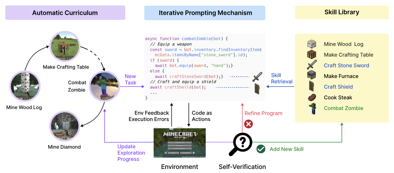
In this paper the "brain" is a large language model (GPT-4), and it is able to interact with both the game world, and a code library where the LLM can both read, write and organize information.

By doing so the agent is capable of using skills and information that has been written in the distant past. This effectively increases the context length of the language model.

Overall, these examples showcase how different approaches and topologies can enhance data coherence in systems, resulting in more meaningful and contextually rich outputs.

Conclusions

We have shown how the right topology for cell communication is a necessary feature for long range coherence by framing the problem of data generation as interactions of multiple sub-units.

Biological systems have long exploited self-organization and indeed possess the right topology to be able to self-organize, furthermore we showed how current NLP algorithms don't possess the needed topology and because of that are incapable of generating long and coherent text.

The same requirements needed for generating coherent text apply to agents trying to navigate a problem space by performing a series of actions, thus all the results also apply in the field of reinforcement learning if the agent has to remember past actions in order to correctly act in the future.

However, since disorder can lead to glassy dynamics, we calculated the memory capacity of self-organizing systems made only by local interactions.

We also showed how an agent with limited context (such as a transformer based LLM) can in principle be able to extend their context by deliberately interacting with the external environment and how biological organisms learned this skill to be able to retain information for a long time.