How to Predict Uncertainty

A small blog post on how to teach your model to output their prediction-confidence

In classification, confidence is built into the output: the model predicts a probability distribution over classes. When it is confident, the distribution becomes sharp (one class gets most of the mass). When it is uncertain, the distribution becomes flatter.

Figure 1: Same task, different confidence: sharp probabilities indicate certainty, flatter probabilities indicate ambiguity.

But what happens when the target is not a class, but a vector?
With plain MSE, the model outputs only a point estimate, so confidence is not explicit.

Can a regression model predict both the target value and its uncertainty?

The answer is yes! To recover that notion of confidence in regression, we make the model predict a full distribution, not just its mean.

The Core Formulation

Suppose we have some datapoints and we want to predict the ground truth probability $p(y|x)$.

We don't have direct access to $p$, so we are going to approximate $p(y|x)$ with $q(y|x)$ where is a gaussian where the mean and the variance are learned functions $\mu_\theta(x)$ and $\sigma_\phi(x)$ $$ q(y|x) = \frac {1}{\sqrt{2 \pi \sigma_\phi^2}} \exp -\frac{(y-\mu_\theta)^2}{2\sigma_\phi^2} $$ The loss is simply going to be the negative log likelyhood of $q(y|x)$ $$ L = -\log q(y|x) = -\log\left[\frac {1}{\sqrt{2 \pi \sigma_\phi^2}} \exp -\frac{(y-\mu_\theta)^2}{2\sigma_\phi^2}\right] $$ Doing some simple calculations, get that the loss is equal to (up to some constant) $$ L = \log \sigma_\phi + \frac{(y-\mu_\theta)^2}{2\sigma_\phi^2} $$ As a sanity check, you can see that if we consider $\sigma_\phi$ to be a constant, we recover the $L_2$ loss.

Now let's train a model with this loss!

Toy model

Suppose that the average value of $y$ is linearly dependent on $x$, i.e., $\mu = a x + b$, and the dispersion around the mean is also linearly dependent on $x$, i.e., $\sigma = |c x + d|$. This means that $$ p(y|x) = \mathcal{N}\!\left[a x + b, (c x + d)^2\right] $$

Linear Regression with Uncertainty

Figure 2: gray points are sampled data, orange is ground truth $p(y|x)$, blue is the model estimate $q(y|x)$.

Start Training Regenerate Data Reset Params

---

Mean Parameters

$a_\theta$: 0.10| 2.00

$b_\theta$: 0.00| 0.00

Sigma Parameters

$c_\phi$: 0.40| 1.00

$d_\phi$: 0.20| 0.20

As you can see the model is able to describe perfectly the ground truth probability distribution by minimizing the loss. Now let's analyze the math to get a better insight on why this is the case.

Properties of this Loss

From the loss in equation , the minimizer with respect to $\sigma_\phi$ is obtained by setting the derivative to zero: $$ \frac{\partial L}{\partial \sigma_\phi} = \frac 1{\sigma_\phi} - \frac {(y-\mu_\theta)^2}{\sigma_\phi^3}=0 $$ And we get that the loss is at the minimum when $$ \sigma_\phi^2 = (y-\mu_\theta)^2 $$ This means that $\sigma_\phi$ learns to estimate the expected prediction error! On the other end, if we calculate the gradient with respect to $\mu_\theta$ we get $$ \frac{\partial L}{\partial \mu_\theta} = \frac{y-\mu_\theta}{\sigma_\phi^2} $$

This means that the gradient to find the expected value of $y$ is exactly the same as the one of the $L_2$ loss, but here each sample is weighted by the expect sample error $\sigma_\phi$- Which is exactly what you want!

Stable Implementation

The problem with equation is numerical stability around $\sigma_\phi\approx 0$. To solve this we can predict log-variance instead of standard deviation directly. Let $l_\phi = \log\sigma_\phi^2$. Then the trainable form of equation becomes: $$ L = l_\phi + (y-\mu_\theta)^2 e^{-l_\phi} $$ This avoids numerical issues from explicit division and logarithms on small values.

Real-World problems

This theory has been around for quite a while . Curiously, there are very few example of such approach being used in the image processing literature , but actually it can be applied very easly! Here is a Video-VAE that I've trained. As you can see it works pretty well!

Figure 3: The first row represents the original frames $y$, the second row the reconstructed image $\mu_\theta$ and the third row the uncertainty $\sigma_\phi$.

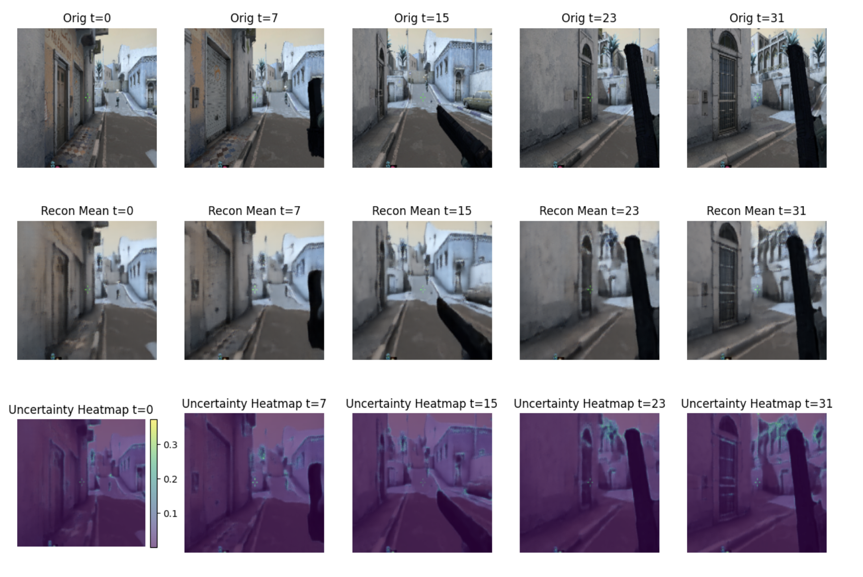
As you can see the areas where the model is less precise (mainly some edges and tree leafs) are highlighed in the uncertanty heatmap.

The way this is done implementation-wise is super simple: you just output 6-channels per pixel: one for the RGB values and one for their uncertainty.

Conclusion

Uncertainty-aware regression gives the model two outputs that matter in practice: prediction and confidence. This small change allows us to estimate pixel-wise uncertainty.