Curiosity-Driven Tree Search

This is the second blog post of my series of "mathematical foundations of curiosity"

In the previous blog post we examined what curiosity is in the context of the $K$-armed bandits problem. Here we are going to show how you can make a scalable tree-search algorithm out of it, and use it for board games such as tic-tac-toe, hex, chess and go.

This line of search-based game-playing systems includes AlphaGo, AlphaZero, and MuZero. In this blog post, I'm going to show you how it is possible to create an algorithm competitive with AlphaZero from first principles.

Figure 1: Curiosity-based search with an maximaly dumb model. Over time it finds the best move. Wanna know how it works? Read the blog!

Games as unfair coin tosses

Suppose two players, $A$ and $B$, are given a particular board state $s$. We want to predict the probability that each player will win. From simplicity, we are going to ignore draws to make the explanation simpler

The game rules may be deterministic, but the players, are not. Each follows a policy, $\pi_A$ and $\pi_B$. From the current position, the eventual winner therefore behaves like the outcome of an unfair coin. Mathematically, you can show how you can derive the probability of $A$ winning from state $s$ under the two policies the following way:

Let $\tau=(s_0,a_0,s_1,a_1,\ldots)$ denote a complete game and let $i_t\in\{A,B\}$ be the player who moves at time $t$. The probability that $A$ wins from state $s$ under the two policies is $$ p_A(s;\pi_A,\pi_B) =\sum_{\tau\,:\,s_0=s} \mathbf{1}\{\operatorname{winner}(\tau)=A\} \prod_t \pi_{i_t}(a_t\mid s_t). $$ Thus, if draws are excluded, the winner $Y$ satisfies $p(Y\mid s,\pi_A,\pi_B)\sim\operatorname{Bernoulli} (p_A(s;\pi_A,\pi_B))$, where $Y=1$ means that $A$ wins and $1-p_A$ is the probability that $B$ wins.

Figure 2: Here, the true odds $p_A(s)$ are shown by the solid orange line, while the blue curve is the model’s prediction $\operatorname{Beta}\!\left(\cdot | \theta \right)$ and the solid blue line marks its mean. The model receives a lower loss when the curve places more density at the true odds.

Let's say that we want to train a NN that predicts the probability $p_A(s)$ of the player $A$ winning given a board state $s$. What would be the correct way of parametrizing the problem?

The thing we want to minimize is the Negative Log-Likelihood (NLL) of the actual real-world odds of $A$ winning. For this, we use a Beta distribution: the conjugate prior to the Bernoulli likelihoodThe Beta distribution is a family of distributions over a probability $p\in(0,1)$. Its density is $$ f(p;\alpha,\beta) =\frac{p^{\alpha-1}(1-p)^{\beta-1}}{B(\alpha,\beta)}, \qquad \alpha,\beta>0. $$
Its two parameters have an intuitive decomposition: $$ \underbrace{\frac{\alpha}{\alpha+\beta}}_{\text{mean: predicted odds}}, \qquad \underbrace{\alpha+\beta}_{\text{concentration: confidence}}. $$
This makes the Beta distribution a natural representation of uncertainty about an unknown Bernoulli probability. It has exactly the right support, and it expresses both where the win probability is believed to lie and how certain that belief is.

It is also conjugate to the Bernoulli likelihood. If $$ p\sim\operatorname{Beta}(\alpha,\beta) $$ before observing any new games, then after $w$ wins by $A$ and $\ell$ losses, $$ p\mid\text{data} \sim\operatorname{Beta}(\alpha+w,\beta+\ell). $$
In other words, every win adds one unit of evidence to $\alpha$, and every loss adds one to $\beta$. In this model the network outputs these two positive parameters for each board state, so its prediction is a full distribution over the latent win probability rather than only a point estimate. $$ \mathcal L(s)=-\log\operatorname{Beta}\!\left(p_A(s) | \theta \right). $$ Where $\theta$ are trainable model parameters.

This NLL lets us learn a full predictive distribution, which gives us an estimate of the model's uncertainty.

A toy example

Suppose our dataset contains several board positions. For every position, we let the same two players play from there many times. Once we have enough games, we'll have reasonably accurate empirical estimates of $p_A$ to use as training targets for our model.

Figure 3: A toy dataset of chess positions. Select a board to compare the win rate estimated from repeated games with the model’s prediction. The positions are adapted from the Lichess “10 Immortal Games” study; all odds and predictions are made up.

In principle, a model can learn the mapping from a board state to these outcome odds. After training, we can give it a position it has never seen and ask it to predict how games between players like $A$ and $B$ would usually end from that position.

Let's be clear: this is not how you train a chess engine. The point of this section was to show how a Beta distribution can represent both a prediction and its uncertainty.

What search does

A tree-search algorithm estimates the probability of winning for each possible next move, assuming both players play optimally.
Because the optimal strategy is often unknown, the algorithm is uncertain about its evaluation, so its estimates must be represented as probability distributions.

Figure 4: Search starts from the network’s broad Beta prediction. As it gathers evidence, the output becomes more concentrated, expressing greater confidence in the estimated win probability.

In a tree-search algorithm, the network provides an initial distribution $q_\theta$ as a starting guess; search improves it, and the improved prediction $q_\textrm{search}$ becomes the network's training target.

$$ L = D_{\mathrm{KL}}\!\left(q_{\mathrm{search}} \;\middle\|\; q_\theta\right). $$

To me, this really feels like how search should work: it should produce a more precise evaluation of the position!
Furthermore, the loss should be the amount of information gained from the search process, as a matter of fact the unit of measurement should be bits! This loss is effectively the same as the NLL shown in the previous section $$ \mathbb E_{q_{\mathrm{search}}}\!\left[-\log q_\theta\right]= D_{\mathrm{KL}}\!\left(q_{\mathrm{search}}\middle\|q_\theta\right) +\underbrace{H\!\left(q_{\mathrm{search}}\right)}_{ \text{has zero gradient}}. $$ If the tree-search algorithm proves that one of the players has a forced win opportunity, then the target becomes a Dirac delta function.

But how does search work precisely?

Move selection

Figure 5: The parent node is represented by the value distribution $V$, the children by $Q_a$ distributions.

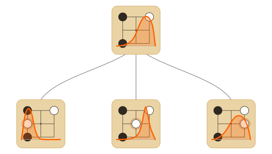
Let's suppose we only have a root node with an initial guess about its value distribution $V$ and some children with value distributions $Q_a$. We want to know is:

What is the probability that a given action $a$ is the best action $a^\star$?

This can be written mathematically as follows:

$$ \mathbb P(a=a^\star) = \mathbb P\left(q_a \geq q_b\;\;\forall b\neq a\right), \quad q_a\sim Q_a. $$

This is the same question we asked in the first post when studying the $K$-armed bandit problem.

We can compute the probability that "child $a$ is the best" directly from their densities like so:

$$ \mathbb P(a=a^\star) = \int_0^1 f_a(x) \prod_{b\neq a} F_b(x)\,dx, $$

where $f_a$ is the density of $Q_a$ and $F_b$ is the cumulative distribution function of $Q_b$. This integral is surprisingly GPU-friendly as well! Here is why this integral is GPU-friendly:
Pick a shared grid of $G$ points, $x_1,\ldots,x_G$, and then:

1. Evaluate $f_a(x_g)$ for every action $a$ and grid point $x_g$ at once. This gives one big $A\times G$ table whose entries can be computed in parallel.

2. Turn each row into its CDF $F_a(x_g)$ with a prefix sum—a running numerical integral. GPUs implement these scans efficiently for all actions in parallel.

3. At each grid point we need $\prod_{b\neq a}F_b(x_g)$ for every action. Recomputing that whole product separately for each action would be wasteful. Instead, add the log-CDFs once and subtract the current action's term: $$ S_g=\sum_b\log F_b(x_g), \qquad \prod_{b\neq a}F_b(x_g) =\exp\!\left(S_g-\log F_a(x_g)\right). $$ In practice, zero CDF values are handled separately so that we never literally compute $\log 0$.

4. Finally, multiply by $f_a(x_g)$ and sum over the grid for every action at the same time. The whole calculation takes $O(AG)$ work instead of the naive $O(A^2G)$.

Empirically you also found we can get a quite good approximation of this integral using a shared grid of just $G=21$ points, and it's much faster than monte carlo!

However, if we just want to do one sample from this distribution we don't even need to evaluate this integral explicitly, we can just do a Thompson-sample: sample one possible value from every child and choose the biggest one.

$$ \tilde q_a\sim Q_a \quad\text{for each }a, \qquad a_{\mathrm{TS}}=\arg\max_a\tilde q_a. $$

As a result, we can sample a policy equal to the probability that each action is optimal under our current beliefs:

$$ \pi(a) =\mathbb P(a=a^\star). $$

This policy is natively curious. A child does not need to have the highest expected value to be worth exploring: it only needs enough uncertainty for there to be a meaningful chance that it is actually the best move

Figure 6: Policy probabilities induced by uncertain value estimates. The model is inherently curious: uncertain beliefs encourage it to explore moves that may appear suboptimal but still have a meaningful chance of being the best.

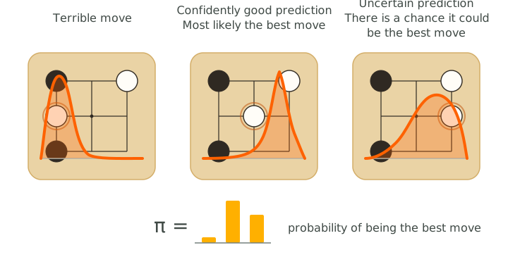
Unlike PUCT, which handles uncertainty indirectly through visit counts, our model predicts its uncertainty explicitly. This allows exploration to be guided by what the model does not yet know, rather than only by how often a move has been examined.

Updating beliefs

Exploring a child is useful only if what we learn there can change what we believe about its parent. Now we are going to see how we can use the information of the child to update our beliefs about the parent.

The previous section gave us

$$ \pi(a)=\mathbb P(a\text{ is the best move}). $$

We reuse those probabilities to combine the current beliefs about the moves:

$$ \bar Q=\sum_a \pi(a)Q_a. $$

Thus, a move that is very likely to be best has a large influence on the position’s value. An uncertain move can still matter when there is a meaningful chance that it is best.

Figure 7: Three action beliefs and their probabilities of being the best move. The exact weighted mixture is generally not a Beta distribution; search keeps a Beta-shaped summary by averaging the three parameter vectors with the same weights. I found this approximation to be good enough, and it keeps things simple.

We do not immediately throw away the network’s original prediction. Instead, we blend it with the information obtained from search:

$$ C = (1-\gamma)V + \gamma\bar Q, \qquad \gamma=\frac{n}{\kappa+n}. $$

Here $n$ measures how much search support has accumulated below the position, while $\kappa$ controls how strongly we initially trust the network. This has the same form as a Bayesian update with a Beta prior. A prior with mean $V$ and concentration $\kappa=\alpha+\beta$ can be written as $\operatorname{Beta}(\kappa V,\kappa(1-V))$. After $n$ Bernoulli observations with empirical mean $\bar Q$, its posterior mean is $$ \frac{\kappa V+n\bar Q}{\kappa+n} =\frac{\kappa}{\kappa+n}V+\frac{n}{\kappa+n}\bar Q. $$ Thus $\kappa$ behaves like a prior sample size: when $n=\kappa$, the prior and the new evidence receive equal weight, while a larger $\kappa$ means that more evidence is needed to move away from the network's prediction.

The update here is only pseudo-Bayesian. Search backups are not literally independent Bernoulli observations, so $n$ is best understood as an effective amount of search evidence. We borrow the weighting rule and its prior-strength interpretation without claiming that the result is an exact Bayesian posterior.

Building the tree

Now we have everything needed to build a search tree. Thompson sampling tells us where to look, while the update rule tells us how to propagate the information we find back to the rest of the tree. Search builds the tree by repeatedly combining these two operations.

$$ \text{sample downward} \longrightarrow \text{expand one position} \longrightarrow \text{update beliefs upward}. $$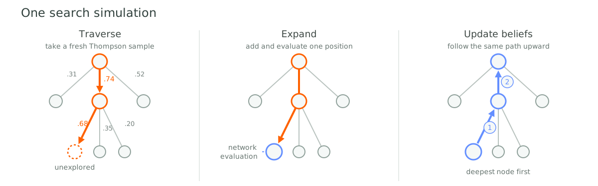

Figure 8: One search simulation. In the first panel, Thompson sampling draws one value from each distribution and selects the largest one, choosing a path from the root to an unexplored move. Search evaluates at most one new position, then updates beliefs along the same path from the deepest node back to the root.

def search_simulation($root$):

$s \leftarrow root$

$path \leftarrow [\,]$

$a \leftarrow$ thompson_sample$(s)$

while $(s,a)$ is explored:

append $(s,a)$ to $path$

$s \leftarrow$ child$(s,a)$

$a \leftarrow$ thompson_sample$(s)$

append $(s,a)$ to $path$

$s' \leftarrow$ expand$(s,a)$

for each $(s,a)$ in reverse$(path)$:

$Q_a \leftarrow$ belief of child$(s,a)$

$C \leftarrow$ update_belief$(V,\{Q_b\})$

return tree

The whole procedure can be summarized in the algorithm to the side right here.

Typically, predictions become sharper as the search moves deeper into the tree because positions farther along in the game are, on average, easier to evaluate.

Empirically, this appears as an increasingly concentrated distribution over moves and a corresponding decline in policy entropy.

What about draws?

With only wins and losses, the outcome is Bernoulli: once we know $p_{\mathrm W}$, the other probability is fixed by $p_{\mathrm L}=1-p_{\mathrm W}$. A Beta distribution is therefore enough to describe our uncertainty about the single free probability.

A draw adds a third possible outcome, so we use its multi-outcome generalization: the Dirichlet distribution.

Figure 9: A Beta distribution places density along the one-dimensional win–loss line. Once draws are possible, the belief lives on a two-dimensional simplex: every point in the triangle is one complete win–draw–loss probability vector. Darker filled contours indicate higher probability density, while the magenta marks show the means of the example distributions.

The Dirichlet distribution has virtually all the same properties as the Beta distribution, so all the math we talked so far remains basically the same.

The triangle in the tic-tac-toe demo visualizes this Dirichlet distribution: each point represents a different combination of win, draw, and loss probabilities.

Results

Board size

6 × 6

Figure 10: Players alternate claiming empty cells. Blue connects the blue left and right edges; red connects the red top and bottom edges. The first unbroken path wins, and Hex cannot end in a draw.

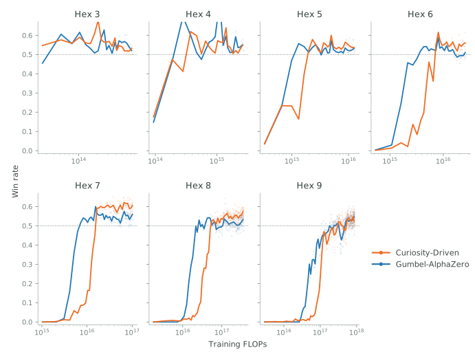
I decided to compare this Curiosity-Driven tree-search algorithm against Gumbel-AlphaZero (the latest iteration of the AlphaZero algorithm by Google-DeepMind)

For the experiments I was inspired by the paper "Scaling Scaling Laws with Board Games", where the author chose to train several models with different hex board sizes from $3\times3$ through $9\times9$ and measured scaling laws for both algorithms.

And it's scalable and competitive with Gumbel-AlphaZero!

Figure 11: Win rate against a roughly optimal-play baseline as a function of neural-network FLOPs. Color denotes board size; faint points are raw evaluations and solid curves are time-averages. The dotted line marks a 50% win rate.

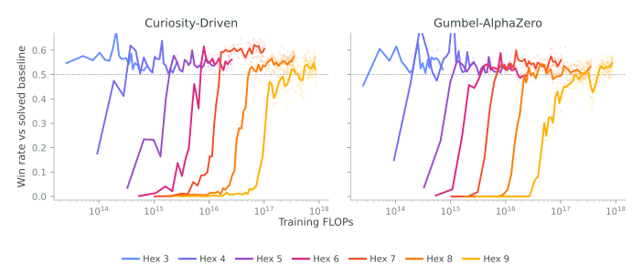
Gumbel-AlphaZero tends to converge faster, while Curiosity-Driven seems to reach slightly better final performance (althought it's pretty negligible).

Figure 12: Matched-board comparison of Curiosity-Driven and Gumbel-AlphaZero.

Figure 13: Prediction entropy for Curiosity-Driven agents as a function of training FLOPs.

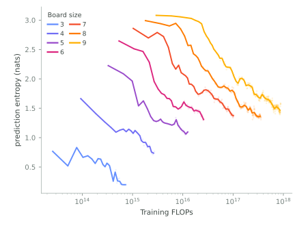
Another interesting graph is the entropy of the predictions as the training goes on. You can clearly see how it learns smootly to predict with higher and higher accuracy (Figure 13).

Experimental details

I used a JAX-native stack made of:

• PGX for fast and parallelizable environments;
• MCTX as the initial version of the tree-search algorithm;
• A custom adaptation of mctx for Curiosity-Driven search.

Self-play/training batch sizes were 4,096/1,024; the network was a 128-channel ResNet with six blocks, trained with Muon at a fixed $5\times 10^{-3}$ learning rate.

Conclusion

The algorithm follows from a small set of simple axioms with minimal additional assumptions. I prioritized mathematical elegance over raw performance: a principled foundation can always be optimized later.

We have seen how the notion of Curiosity, introduced in the first post of this series, can be generalized into a complete and scalable tree-search algorithm that performs competitively with AlphaZero.

If you want to work on this kind of research and are curious about this stuff reach out! 🐝